Curve Fitting

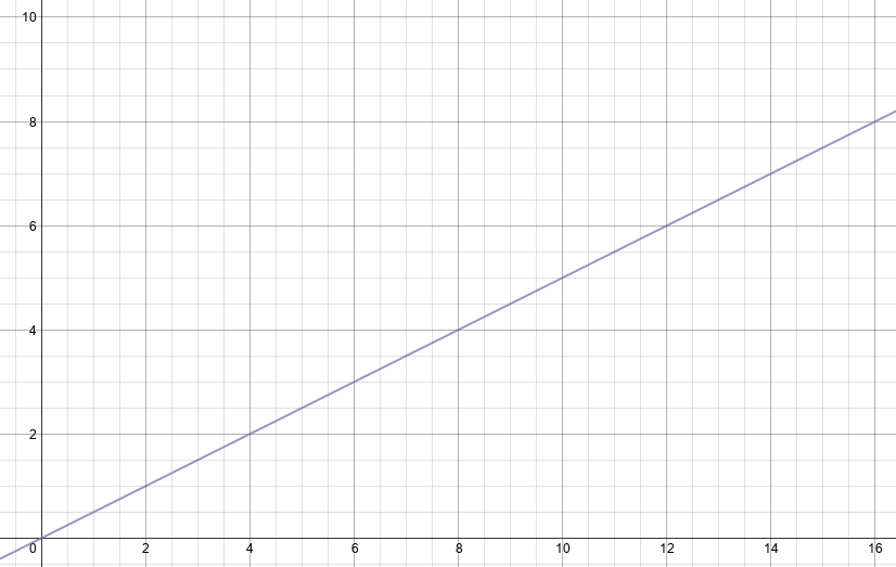
Here is a simple technique to modify linear data points to a curve of your choice. If your function looks linear like this:

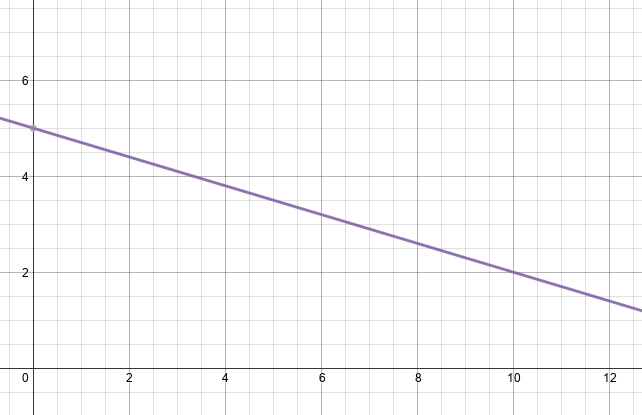
or even has an inverse linear form like this:

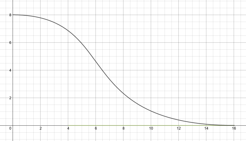
And you want to instead map it to a curve that accentuates the initial values and suppresses the tail:

or has an exponential drop at the end points like this:

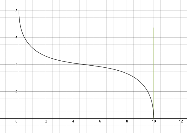
then, Cubic Bezier curves can be used to achieve the desired transformation. A Cubic Bezier curve is given by:

B(t) = (1 - t)³P₀ + 3(1 -t)²tP₁ + 3(1 -t)t²P₂ + t³P₃

Here P₀, P₃ are the end-points of the curve and P₁ and P₂ are control points. A Cubic Bezier curve, at the starting point is always tangential to the line segment P₀, P₁ and in the direction of P₀, P₁. At the endpoint, the curve is tangential to P₂, P₃ and is in the direction of P₂, P₃. You can play around with various Cubic Beziers shapes at desmos.com.

When implementing a Cubic Bezier curve, the first oddity you will encounter is the fact that unlike polynomial equations, the Bezier does not give you y-coordinates as a function of x-coordinates. Instead, it independently gives you x and y coordinates as a function of a parameter t which varies from 0 to 1. When t = 0, the curve is at point P₀ and when t = 1, the curve is at point P₃. Worse, when you vary t linearly, you do not get linear increments of x. Instead, you get linear increments along the curve’s length. In fact, it is this property of Bezier curves that makes them suitable as easing functions for animations. By constructive a Cubic Bezier with steep starting and ending slopes, you can get a slow start in the x axis followed by an acceleration in the middle and a gradual slowdown towards the end. But for mapping a traditional function of the form y = f(x), we would like to transform the Bezier to a similar function.

There is no simple mathematical way to achieve this given expressions like t² and t³ in the equation. Instead, one can approximate a solution by doing a binary search along t, computing the corresponding x until we are within a tolerance limit. At that point, the value of y can be computed. The gist below shows a Java program to do that. In addition, the program allows you to pre-compute y = Bezier(x) for x = (start, end) in specified increments.

The class above can be extended to create a composite Cubic Bezier curve fitting algorithm that combines multiple Cubic Bezier curves to model any shape you want to create.